Summary
This report was produced for a course in stochastic processes. I explored how birth-death processes, a type of continuous time Markov chain, could be applied to epidemic modelling. I found that framing epidemic outbreaks as birth-death processes allows one to estimate the probability of a major epidemic occurring, and the subsequent duration and final sizes. The projections in the report are not meant to be accurate as the models made numerous unrealistic assumptions - this was just an academic exercise in modelling.
Introduction
COVID-19 has been declared a global pandemic by the WHO (Cucinotta and Vanelli 2020), and a lot of attention has been focused on the development of epidemiological models to understand its dynamics. The Susceptible-Infectious-Removed (SIR) epidemic model is a well-known model that captures the dynamics of an epidemic (McKendrick 1925). A SIR model comprises of three compartments, \(S\), \(I\), and \(R\) that represent the number of people in a population who are susceptible to, infected by and have recovered from a disease (and are therefore immune). The transitions between the states are determined by ordinary differential equations (ODEs) detailed in the equations below.
\[\frac{dS}{dt} = - \beta I\frac{S}{N}\]
\[\frac{dI}{dt} = \beta I\frac{S}{N} - \gamma I\] \[\frac{dI}{dt} = \gamma I \]
where \(\beta,\ \gamma\) represent the rate of transmission and rate of recovery of the disease. The basic reproduction number \(R_{0} = \beta\text{/}\gamma\) refers to the expected number of secondary cases directly generated by one case in a fully susceptible population, in the absence of any intervention.
The model described above is deterministic and does not have any inherent randomness. In other words, given certain parameters, the model will only output one fixed trajectory of an epidemic. Deterministic models are valid for sufficiently large populations, but are unable to capture typically stochastic phenomena like extinction (Rock et al. 2014). In situations where the number of infectious individuals is small or when the variability in transmission and recovery impacts the epidemic outcome, the randomness in stochastic models are more appropriate (Allen 2017).
The objective of this project is to explore the stochastic SIR epidemic model in the framework of a continuous-time Markov chain – more specifically, a birth-death process (BDP). This includes explaining the theoretical formulation of an SIR BDP, before fitting it onto COVID-19 case data and conducting simulation-based inference from the models.
Methods
SIR as a Continuous-Time Markov Chain & Birth-Death Process
To formulate the SIR model as a continuous-time Markov chain (CTMC), two discrete random variables \(S\) and \(I\) are defined to record the number of susceptible and infectious individuals in a homogeneously mixed closed population of size \(N\), such that:
For a small period of time \(\Delta t\), the transition probabilities for the stochastic process are:
\[\begin{align*} P_{\left( s,i \right),\left( s + k,i + j \right)}&\left( \Delta t \right) =\\ &P\lbrack(S(t + \Delta t),\ I(t + \Delta t) = (s + k,i + j)|(S(t),I(t) = (s,i)\rbrack \end{align*}\]
The CTMC is a time-homogeneous process, in that the transition probabilities do not depend on specific values of \(t\) but only on the time between events, \(\Delta t\). Furthermore, according to the Markov property, the state of the process at time \(t + \Delta t\) depends only on the state at time \(t\) and not any states prior to \(t\). A birth-death process (BDP) is a special case of the CTMC where the state variable can only increase or decrease by 1. Under the assumption of a closed population, the rate of births, deaths and immigration in reality is negligible and do not affect the epidemic dynamics. Mathematically, this means that \(N - S\left( t \right) - I\left( t \right)\) remains constant. Thus, the only transition probabilities are related to infection and recovery, as summarised below.
| Event | Change \(\left( \Delta S,\Delta I \right)\) | Probability |
|---|---|---|
| Infection | \[\left( - 1, + 1 \right)\] | \[\beta i\frac{s}{N}\Delta t + o\left( \Delta t \right)\] |
| Recovery | \[\left( 0, - 1 \right)\] | \[\text{γi}\Delta t + o\left( \Delta t \right)\] |
The model is initialised at time \(t = 0\) for some infected individuals \(I\left( 0 \right) = i > 0\) and \(S\left( 0 \right) = N - i\) susceptible individuals, and the epidemic ends when \(I\left( t \right) = 0\). In other words, the states \(\left( s,0 \right)\) for all possible \(s\) are absorbing states.
Parameter estimation
Data
The dataset used in this paper was sourced from the Johns Hopkins University COVID-19 repository (CSSE 2020). The repository contains data on the daily number of confirmed cases, deaths and recovered cases for every country affected by the pandemic and is updated daily.
Maximum Likelihood Estimation
The likelihood for a continuously observed BDP is formulated as such:
\[L = \prod_{k = 0}^{\infty}{\lambda_{k}}^{U_{k}}{\mu_{k}}^{D_{k}}\exp\left\lbrack - \left( \lambda_{k} + \mu_{k} \right)T_{k} \right\rbrack\]
where \(U_{k},D_{k}\) are the number of up (arrivals) and down (removals) steps respectively, and \(T_{k}\) is the total time spent in state \(k\) over all visits to \(k\) (Crawford and Suchard 2014). \(\lambda_{k},\mu_{k}\) represent the instantaneous rate at which arrivals and removals occur. For simplification, the arrival and removal rates are assumed to be linear \(\lambda_{k} = k\lambda,\mu_{k} = k\mu\), and this process is also known as the Kendall process. In the context of an epidemic, an arrival refers to an infection while a removal could refer to either a recovery or death.
However, this likelihood is difficult to evaluate analytically because the number of COVID-19 cases is only reported at discrete time points (daily) rather than over a continuous time. When a BDP is sampled discretely such that only \(X\left( 0 \right) = a\) and \(X\left( t \right) = b\) are observed, the quantities \(U_{k}\), \(D_{k}\), and \(T_{k}\) are unknown for every state \(k\), and the log-likelihood cannot be maximised without them (Crawford, Minin, and Suchard 2014). Previous studies have shown that a continuous-time BDP process observed at equidistant points form a Galton-Watson process but the transition probabilities are complex and direct maximum likelihood estimation did not seem feasible (Keiding 1975).
Therefore, a data augmentation technique was applied to approximate a continuously observed BDP. This involved splitting the daily reported case number into individual jumps of \(+ 1\) or \(- 1\) distributed by a uniform distribution with a width equal to \(1\text{/}n\), where \(n\) refers to the number of cases that occurred on that day.
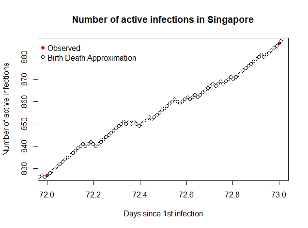
An example of the result is illustrated above. On the 73rd day since the first case in Singapore, there were 75 new cases and 16 recoveries reported. The data augmentation process split the time interval (72,73) into 91 bins and computed 75 up steps and 16 down steps at random. Conducting this data augmentation technique on the daily case data enabled the maximisation of the likelihood function to estimate the transition rates \(\lambda,\mu\). These parameters can be thought of as the transmission and recovery rate \(\beta,\gamma\) in the SIR model although they are not completely the same since \(\mu\) includes both deaths and recoveries. Analogously, \(\lambda\text{/}\mu\) is a crude estimate of \(R_{0} = \beta\text{/}\gamma\). The maximum likelihood (ML) estimates for \(\lambda,\ \mu\) and their respective standard errors are summarised below.
| Country | \(\lambda_{MLE}\) | SE | \(\mu_{MLE}\) | SE | \(\lambda/\mu\) | |||
|---|---|---|---|---|---|---|---|---|
| France | 0.100 | 2.06 \(\times\) 10-7 | 0.0371 | 1.25 \(\times\) 10-7 | 2.71 | |||
| Singapore | 0.138 | 7.78 \(\times\) 10-6 | 0.0163 | 2.67 \(\times\) 10-6 | 8.46 | |||
| South Korea | 0.0409 | 7.77 \(\times\) 10-7 | 0.0319 | 6.86 \(\times\) 10-7 | 1.28 | |||
| Sweden | 0.0729 | 1.37 \(\times\) 10-6 | 0.0106 | 5.21 \(\times\) 10-7 | 6.88 | |||
| Thailand | 0.0766 | 7.67 \(\times\) 10-6 | 0.0547 | 6.48 \(\times\) 10-6 | 1.4 |
A limitation of the linear BDP is that it assumed that rates \(\lambda,\mu\) are constant throughout the outbreak. This is not likely to be true in reality as the rates are very sensitive to day-to-day changes in the number of reported cases. For example, while Singapore has been relatively successful in managing the epidemic initially, the recent spike in cases reported in Singapore around 20th April (Griffith 2020) have resulted in a sharp increase in \(\lambda\). Thus, the estimates tend to vary greatly depending on the state of the epidemic at the time.
As such, a more accurate interpretation of \(\lambda,\ \mu\) is a reflection how successful the countries have been in controlling the epidemic. Low values of \(\lambda\) indicate a success in reducing the rate at which infections occur. The countries highlighted above were selected to highlight a range of scenarios for different points of the outbreak. South Korea has been shown to have largely controlled the epidemic (Normile 2020), while the other countries are still dealing with a large number of cases. The relative low rates of \(\lambda,\ \mu\) for South Korea support this statement. However, it should be noted that the removal rate \(\mu\) includes both recoveries and deaths, so while Singapore and Sweden appear to have very high \(\lambda\text{/}\mu\) (which is analogous to \(R_{0}\)), their situation may not be as bad as in France, which has a relatively high \(\mu\) that includes a large number of deaths (Ward 2020).
Despite their simplification, the MLE estimates for \(\lambda,\mu\) may still serve to highlight how different epidemics are expected to progress through simulation.
Simulation-based Results
The estimated model parameters were used to simulate various trajectories of the epidemic in the respective countries. The Gillespie algorithm allows for the simulation of possible solutions of a stochastic equation (Gillespie 1977) and can be applied in this scenario. The pseudocode of the algorithm is provided below.
|
The stochastic nature of each epidemic allows some inference to be made about the paths of the epidemic. These include the i. probability of a major outbreak, ii. the final size and iii. duration of the epidemic. For each country, a total of 100 simulations were run until \(I\left( t \right) = 0\) and the extinction times \(inf\text{\{}t > 0|I(t) = 0\text{\}}\) and final sizes of the epidemic were recorded. The simulated results were then compared with their deterministic ODE counterparts.
Probability of Major Outbreak
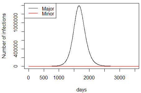
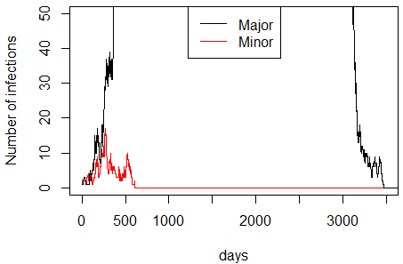
Due to the stochasticity of the birth-death process, there is a possibility of infections being removed before a major epidemic occurred, so not all processes will lead to major outbreaks. Here, a major epidemic is characterised as one that has a generally longer duration and substantially greater number of cases than a minor epidemic (Tritch and Allen 2018). Theoretically, only minor epidemics occur when \(R_{0} < 1\) and given \(R_{0} > 1\), the probabilities of a minor and major epidemic are \(\left( 1\text{/}R_{0} \right)^{i}\) and \(1 - \left( 1\text{/}R_{0} \right)^{i}\) respectively, where \(i\) refers to the initial number of infected individuals (Whittle 1955). The distinction between the two types of epidemics is illustrated nelow at different scales.
The probability of a major epidemic occurring can be approximated by the proportion of simulated Markov chains that resulted in a major epidemic. The results are summarised below.
| Country | Theoretical \(P(\text{major})\) | Estimated \(P(\text{major})\) |
|---|---|---|
| France | 0.631 | 0.84 |
| Singapore | 0.881 | 0.85 |
| South Korea | 0.219 | 0.24 |
| Sweden | 0.855 | 0.86 |
| Thailand | 0.286 | 0.5 |
The estimated probability of a major outbreak is largely correlated to the theoretical value \(\left( R^{2} = 0.81 \right)\), although the strength of association varies. The variance could be attributed two sources: firstly, \(\lambda\text{/}\mu\) is only a crude estimator of \(R_{0} = \beta\text{/}\gamma\) and secondly, the stochastic nature of the simulations results in a variable probability of major outbreak. Only the second source can be addressed by increasing the number of simulations, which also increases the time and computational cost.
The results are consistent with the understanding that South Korea has been successful in managing the outbreak and effectively reduced the probability of a major outbreak occurring. On the other hand, the probability of major outbreaks occurring in the other countries are substantially higher.
Final Size
The final size of the outbreak refers to the total number of people expected to be infected by the disease. Bayes’ rule can be leveraged to estimate the final size based on the outcome of the simulated epidemics.
\[E\left\lbrack \text{final size} \right\rbrack = E\left\lbrack \text{final size} \middle| \text{major} \right\rbrack P\left( \text{major} \right) + E\left\lbrack \text{final size} \middle| \text{minor} \right\rbrack P\left( \text{minor} \right)\]
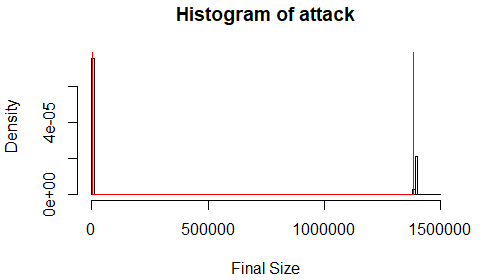
The typical distribution of final sizes is illustrated above. The distribution is characteristically bimodal with the final size depending on whether a minor or major epidemic occurred. The simulation results are summarised below and compared with the final size of the deterministic models.
| Country | \(E[\cdot\| ext{major}]\) | \(E[\cdot\| ext{minor}]\) | \(E[ext{final size}]\) | % | ODE | % |
|---|---|---|---|---|---|---|
| France | 1.73\(\times\) 107 | 3.25 | 1.44\(imes\) 107 | 21.9 | 1.71\(\times\) 107 | 26 |
| Singapore | 3.68\(\times\) 106 | 1 | 3.12\(\times\) 106 | 53.4 | 3.67\(\times\) 106 | 62.8 |
| South Korea | 1.39\(\times\) 106 | 2.54 | 3.35\(\times\) 105 | 0.652 | 1.36\(\times\) 106 | 2.65 |
| Sweden | 5.79\(\times\) 106 | 1.36 | 4.98\(\times\) 106 | 49.4 | 5.79\(\times\) 106 | 57.4 |
| Thailand | 3.17\(\times\) 106 | 3.22 | 1.58\(\times\) 106 | 2.23 | 3.17\(\times\) 106 | 4.53 |
From the table above, the expected final sizes given that a major outbreak occurred \(E[\cdot|\text{major}]\) are very similar to the deterministic ODE solution. Given that a minor outbreak occurred, the expected final size is extremely small. A possible interpretation of this is that the threshold for a major epidemic occurring is very low, seeing that an outbreak only needs to exceed on average 2-3 infections before it progresses into a large epidemic. This is more likely in a homogenous population where people interact with everyone else on a regular basis but that may not be a realistic setting.
It is also interesting to note the differences in the estimated final size \(E[\text{final size}]\) and the ODE solution. The estimated final sizes are much lower than the ODE solutions because they account for the possibility of no major epidemics occurring. In a way these can be interpreted as more realistic final sizes than the deterministic solution.
Expected Duration
The simulated results also allow one to estimate the duration of the outbreak, or in other words, the extinction time. Most theoretical research has focused on the duration of epidemics conditioned on non-extinction (Tritch & Allen, 2018). However, since the outbreaks were simulated till extinction, this project will only estimate the duration conditioned on extinction. Similar to the final size estimation, a possible simulation-based estimate of duration can be formulated by Bayes rule as such:
\[E\left\lbrack \text{duration} \right\rbrack = E\left\lbrack \text{d}\text{uration} \middle| \text{major} \right\rbrack P\left( \text{major} \right)\ + \ E\left\lbrack \text{duration} \middle| \text{minor} \right\rbrack P\left( \text{minor} \right)\]
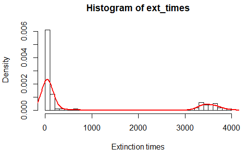
The plot above illustrates the distribution of extinction times. It follows a clear bimodal distribution given the respective outcomes (minor or major outbreaks). The results are summarised below. Since deterministic epidemic models only approach 0 but never become fully extinct, the extinction time for the ODE solution is taken to be when \(I\left( t \right) < 1\text{/}N\), or when there is less than 1 infected person in the population.
| Country | \(E[\cdot\|\text{major}]\) | \(E[\cdot\|\text{minor}]\) | \(E[\text{duration}]\) | ODE |
|---|---|---|---|---|
| France | 909 | 23.4 | 767 | 894 |
| Singapore | 1130 | 7.00 | 965 | 1070 |
| South Korea | 3530 | 60.1 | 893 | 3710 |
| Sweden | 1870 | 20.8 | 1614 | 1780 |
| Thailand | 1640 | 33.5 | 835 | 1630 |
Similar to the expected final size, the expected duration given a major epidemic is close to the ODE solution. The overall expected duration can also be interpreted as a more realistic figure than the ODE solution since it accounts for the probability of only a minor outbreak occurring.
Discussion
The results summarised below illustrate that the selected countries have varied success in managing the COVID-19 pandemic. As mentioned earlier in this report, South Korea seemed to have the epidemic under control. Although the outbreak in South Korea is expected to last for almost as long as any other country, the low rates of \(\lambda,\ \mu\) resulted in the lowest probability of a major outbreak occurring and a substantially smaller estimated final size. However, the model is only able to capture one single epidemic and is unable to forecast future outbreaks which may drastically affect the final size and duration.
| Country | Estimated \(P(\text{major})\) | \(E[\text{final size}]/N\) (%) | \(E[\text{duration}]\) |
|---|---|---|---|
| France | 0.84 | 21.9 | 767.44 |
| Singapore | 0.85 | 53.4 | 965.03 |
| South Korea | 0.24 | 0.652 | 892.59 |
| Sweden | 0.86 | 49.4 | 1613.81 |
| Thailand | 0.50 | 2.23 | 835.4 |
Although the results may seem worrying for Singapore and Sweden, which have an expected 53.4% and 49.4% of their population infected by COVD-19 respectively, it is important to note that these simulations were unable to account for direct public health intervention to reduce disease transmission. In Singapore, where strict physical distancing measures have been introduced, the final size will likely be much lower than expected. Nonetheless, these figures serve to highlight a possible ‘worst case’ scenario where COVID-19 is allowed to transmit freely in a highly mixed, homogeneous population.
Limitations
The BDP model used in this project was mainly limited by its assumptions. Firstly, the model assumed a closed population for each country, and did not consider the effects of births, deaths, or immigration on the epidemic dynamics. This was not a realistic assumption to make since the epidemics have been estimated to last for more than 3 years, during which other demographic effects might have affected the rates of infection and recovery, as well as the population size. From initial reports during the pandemic, it was also understood that immigration was a significant factor in transmission (Pinotti et al. 2020) and should be included in further analysis.
Secondly, for ease of estimating the likelihood, the removal process was simplified to include both recovery and death. This ‘R’ state in SIR is ambiguous and does not capture the severity of the outbreak beyond the number of infected cases. In other words, a country may have a high removal rate leading to a smaller epidemic, but this may or may not be a satisfactory outcome depending on the number of recovered cases relative to deaths. Future work may be undertaken to differentiate between recovered cases and deaths in order to have a clearer representation of the severity of the epidemic.
Furthermore, the Markov property, while useful in simplifying complex phenomena, does not always hold in reality as it does not consider historical trends beyond the past day, when in reality a lot of processes that underpin disease transmission are dependent on time periods much longer than one day. Thus, the BDP model is only useful for early approximations.
It should also be noted that a model is only as good as the data it is fed. The data used in the model only contains reported cases and the proportion of cases reported varies largely depending on different countries’ disease surveillance systems. This may not be representative of the true state of COVID-19 in various countries especially if they lack adequate testing. Nonetheless, the reported number of cases is the most direct way that the state of the epidemic can be observed, even if the statistics may be flawed.
Lastly, since the BDP approximation considers only +1 and -1 transitions between states, it is a time-consuming process to estimate parameters and conduct simulations for countries reported to have a large number of infections. For this reason, countries that were adversely affected by COVID-19 with over 100,000 confirmed cases, including the US, China and Italy, were excluded from this study even though it would have been of value to include them.
Conclusion
In conclusion, this project highlighted an application of birth-death processes to the COVID-19 pandemic. Firstly, it introduced the theoretical formulation of an SIR BDP and its transition probabilities. Secondly, a data augmentation technique was used to overcome the difficulty of computing maximum likelihood estimation on discretely observed BDP. The parameter estimates were then used to simulate outbreaks in different countries, and simulation-based inference was conducted. Lastly, the limitations of applying the BDPs to study the COVID-19 pandemic was discussed at length.
Overall, this project has shown that while the birth-death process is useful in modelling the number of COVID-19 infections, it is largely limited by its assumptions. The model could be refined by introducing more flexibility in order to represent other more complex aspects of the outbreak such as recovery, deaths, demographic trends, and public health interventions.